🚀 Able to supercharge your AI workflow? Strive ElevenLabs for AI voice and speech era!

10 Python One-Liners for Producing Time Collection Options
Introduction
Time collection information usually requires an in-depth understanding to be able to construct efficient and insightful forecasting fashions. Two key properties are vital in time collection forecasting: illustration and granularity.
- Illustration entails utilizing significant approaches to remodel uncooked temporal information — e.g. day by day or hourly measurements — into informative patterns
- Granularity is about analyzing how exactly such patterns seize variations throughout time.
As two sides of the identical coin, their distinction is refined, however one factor is for certain: each are achieved by characteristic engineering.
This text presents 10 easy Python one-liners for producing time collection options based mostly on totally different traits and properties underlying uncooked time collection information. These one-liners can be utilized in isolation or together that can assist you create extra informative datasets that reveal a lot about your information’s temporal conduct — the way it evolves, the way it fluctuates, and which tendencies it reveals over time.
Be aware that our examples make use of Pandas and NumPy.
1. Lag Function (Autoregressive Illustration)
The concept behind utilizing autoregressive illustration or lag options is less complicated than it sounds: it consists of including the earlier remark as a brand new predictor characteristic within the present remark. In essence, that is arguably the best methodology to characterize temporal dependency, e.g. between the present time on the spot and former ones.
As the primary one-liner instance code on this record of 10, let’s take a look at this yet one more intently.
This instance one-liner assumes you will have saved a uncooked time collection dataset in a DataFrame referred to as df, one in every of whose current attributes is called 'worth'. Be aware that the argument within the shift() perform could be adjusted to fetch the worth registered n time instants or observations earlier than the present one:
|
df[‘lag_1’] = df[‘value’].shift(1) |
For day by day time collection information, in the event you wished to seize earlier values for a given day of the week, e.g. Monday, it will make sense to make use of shift(7).
2. Rolling Imply (Quick-Time period Smoothing)
To seize native tendencies or smoother short-term fluctuations within the information, it’s normally useful to make use of rolling means throughout the n previous observations resulting in the present one: it is a easy however very helpful approach to clean generally chaotic uncooked time collection values over a given characteristic.
This instance creates a brand new characteristic containing, for every remark, the rolling imply of the three earlier values of this characteristic in latest observations:
|
df[‘rolling_mean_3’] = df[‘value’].rolling(3).imply() |
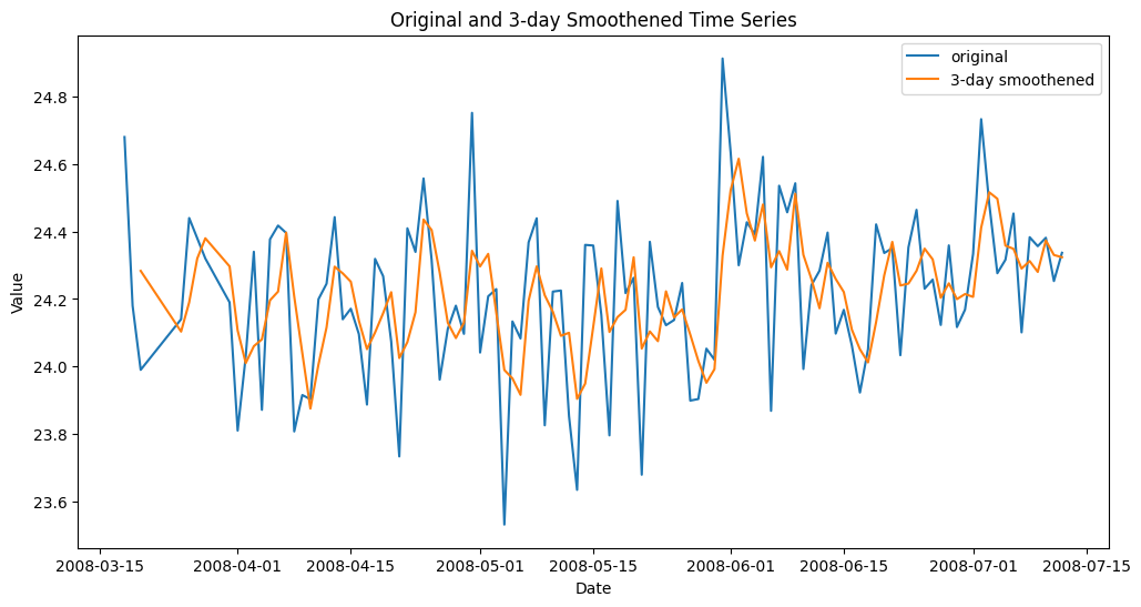
Smoothed time collection characteristic with rolling imply
3. Rolling Commonplace Deviation (Native Volatility)
Just like rolling means, there’s additionally the potential of creating new options based mostly on rolling commonplace deviation, which is efficient for modeling how risky consecutive observations are.
This instance introduces a characteristic to mannequin the variability of the newest values over a shifting window of per week, assuming day by day observations.
|
df[‘rolling_std_7’] = df[‘value’].rolling(7).std() |
4. Increasing Imply (Cumulative Reminiscence)
The increasing imply calculates the imply of all information factors as much as (and together with) the present remark within the temporal sequence. Therefore, it is sort of a rolling imply with a continually growing window dimension. It’s helpful to research how the imply of values in a time collection attribute evolves over time, thereby capturing upward or downward tendencies extra reliably in the long run.
|
df[‘expanding_mean’] = df[‘value’].increasing().imply() |
5. Differencing (Development Removing)
This system is used to take away long-term tendencies, highlighting change charges — necessary in non-stationary time collection to stabilize them. It calculates the distinction between consecutive observations (present and former) of a goal attribute:
|
df[‘diff_1’] = df[‘value’].diff() |
6. Time-Based mostly Options (Temporal Part Extraction)
Easy however very helpful in real-world purposes, this one-liner can be utilized to decompose and extract related info from the complete date-time characteristic or index your time collection revolves round:
|
df[‘month’], df[‘dayofweek’] = df[‘Date’].dt.month, df[‘Date’].dt.dayofweek |
Vital: Watch out and verify whether or not in your time collection the date-time info is contained in a daily attribute or because the index of the info construction. If it have been the index, you might want to make use of this as a substitute:
|
df[‘hour’], df[‘dayofweek’] = df.index.hour, df.index.dayofweek |
7. Rolling Correlation (Temporal Relationship)
This method takes a step past rolling statistics over a time window to measure how latest values correlate with their lagged counterparts, thereby serving to uncover evolving autocorrelation. That is helpful, for instance, in detecting regime shifts, i.e. abrupt and protracted behavioral adjustments within the information over time, which happen when rolling correlations begin to weaken or reverse in some unspecified time in the future.
|
df[‘rolling_corr’] = df[‘value’].rolling(30).corr(df[‘value’].shift(1)) |
8. Fourier Options (Seasonality)
Sinusoidal Fourier transformations can be utilized in uncooked time collection attributes to seize cyclic or seasonal patterns. For instance, making use of the sine (or cosine) perform transforms cyclical day-of-year info underlying date-time options into steady options helpful for studying and modeling yearly patterns.
|
df[‘fourier_sin’] = np.sin(2 * np.pi * df[‘Date’].dt.dayofyear / 365) df[‘fourier_cos’] = np.cos(2 * np.pi * df[‘Date’].dt.dayofyear / 365) |
Permit me to make use of a two-liner, as a substitute of a one-liner on this instance, for a purpose: each sine and cosine collectively are higher at capturing the massive image of attainable cyclic seasonality patterns.
9. Exponentially Weighted Imply (Adaptive Smoothing)
The exponentially weighted imply — or EWM for brief — is utilized to acquire exponentially decaying weights that give increased significance to latest information observations whereas nonetheless retaining long-term reminiscence. It’s a extra adaptive and considerably “smarter” method that prioritizes latest observations over the distant previous.
|
df[‘ewm_mean’] = df[‘value’].ewm(span=5).imply() |
10. Rolling Entropy (Data Complexity)
A bit extra math for the final one! The rolling entropy of a given characteristic over a time window calculates how random or unfold out the values over that point window are, thereby revealing the amount and complexity of data in it. Decrease values of the ensuing rolling entropy point out a way of order and predictability, whereas the upper these values are, the extra the “chaos and uncertainty.”
|
df[‘rolling_entropy’] = df[‘value’].rolling(10).apply(lambda x: –np.sum((p:=np.histogram(x, bins=5)[0]/len(x))*np.log(p+1e–9))) |
Wrapping Up
On this article, now we have examined and illustrated 10 methods — spanning a single line of code every — to extract a wide range of patterns and data from uncooked time collection information, from less complicated tendencies to extra refined ones like seasonality and data complexity.
🔥 Need the most effective instruments for AI advertising and marketing? Take a look at GetResponse AI-powered automation to spice up your corporation!