The best way to use Google Sheets: A newbie’s information

You should use Google Sheets to do virtually something. There’s the intense stuff, like organizing to-do lists, managing leads, and making choices. After which there’s the enjoyable stuff, like taking part in Wordle, simulating a baseball sport, and making customized browser homepages. 

However earlier than you can also make a spreadsheet to trace the variety of minutes your canine has passed by with out being instructed he is an excellent boy—or the stuff that helps you get precise work completed—you need to perceive the fundamentals. 

On this Google Sheets tutorial for rookies, I am going to stroll you thru all the pieces you must find out about how one can use Google Sheets.

Desk of contents:

What’s Google Sheets?

Google Sheets is a spreadsheet app used to prepare, format, and calculate knowledge. It is included as a part of Google Workspace—a collection of related productiveness instruments, together with Google Docs, Google Varieties, and Google Slides. 

You may entry Google Sheets by way of the online, its cell app (out there for Android and iOS), and desktop app (out there solely on Google’s ChromeOS). 

Is Google Sheets the identical as Excel?

Google Sheets and Excel are each spreadsheet apps, so there are a variety of overlapping options. However there are just a few key variations.

• Collaboration. Google Sheets was designed with collaboration in thoughts—that is why it is really easy to share worksheets with varied permission settings. Excel has related collaboration options—for instance, you may add and edit feedback—however the expertise is not as easy as what you get with Google Sheets. 

• Cell limits. Google Sheets has a cell restrict of 10 million, however that pales compared to Excel’s 17 billion cells per spreadsheet. That is what makes Excel the higher device for coping with large knowledge. 

• Formulation. Excel has extra highly effective formulation and knowledge evaluation options, together with built-in statistical evaluation instruments and intensive knowledge visualization choices. Google Sheets, then again, affords a “lite” model of most of those options—however they’re nowhere close to as in-depth.

For an in depth breakdown of how these two apps stack up, try our app showdown: Google Sheets vs. Excel. 

Google Sheets fundamental phrases 

To kick issues off, let’s cowl some spreadsheet terminology you will have to know when utilizing Google Sheets:

• Cell: A single knowledge level or ingredient in a spreadsheet.

• Column: A vertical set of cells.

• Row: A horizontal set of cells.

• Vary: A number of cells extending throughout a row, column, or each.

• Perform: A built-in operation from the spreadsheet app you will use to calculate cell, row, column, or vary values and manipulate knowledge.

• Components: The mix of capabilities, cells, rows, columns, and ranges used to acquire a selected consequence.

• Worksheet (Sheet): The named units of rows and columns that make up your spreadsheet. One spreadsheet can have a number of sheets.

• Spreadsheet: Your entire doc containing your worksheets. 

The best way to create a spreadsheet in Google Sheets

There are 4 methods to create a brand new spreadsheet in Google Sheets. 

From the Google Sheets dashboard 

1. Go to docs.google.com/spreadsheets.

2. Click on Clean spreadsheet. 

From an current Google Sheets spreadsheet

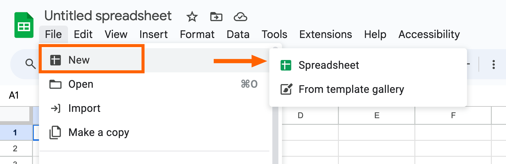
1. With Google Sheets open, click on File.

2. Click on New.

3. Click on Spreadsheet to create a clean spreadsheet or From template gallery to make use of a template. 

   

From Google Drive 

1. Go to drive.google.com.

2. Within the aspect menu, click on New, after which choose Google Sheets. 

3. Choose Clean spreadsheet or From a template. 

Out of your browser’s deal with bar 

1. Along with your browser open, enter sheets.new into the deal with bar. 

2. Press Enter. 

3. A brand new tab with a clean Google Sheet will seem in your browser window.

The best way to add knowledge in Google Sheets

If you create a brand new spreadsheet, you may instantly start typing, and your knowledge will robotically seem within the top-left cell. If you wish to enter knowledge someplace else, click on one other cell and sort away. A blue border will seem across the cell you are typing in to make it simpler to determine which cell you are working with.  

To make it simpler to filter or manipulate knowledge afterward, every cell ought to comprise just one worth—for instance, 100 or Mango.

If you end coming into knowledge right into a cell, you are able to do considered one of 4 issues:

1. Press Enter or return to save lots of the info and transfer to the start of the subsequent row.

2. Press Tab to save lots of the info and transfer one cell to the correct in the identical row.

3. Use your arrow keys (up, down, left, and proper) to maneuver one cell in that path.

4. Click on any cell to leap on to it.

In case you do not wish to sort in all the pieces manually, you can even import knowledge into Google Sheets en masse utilizing just a few totally different strategies:

1. Copy and paste an inventory of textual content or numbers into your spreadsheet.

2. Copy and paste an HTML desk from a web site.

3. Import an current spreadsheet. In case you’re importing knowledge from one other Google Sheet, you can even use the IMPORTRANGE perform to robotically pull in that knowledge and hold issues constant. 

4. Use the fill deal with to robotically populate neighboring cells with knowledge. 

The best way to import knowledge to Google Sheets

If you wish to pull in knowledge from an current spreadsheet, you will first need to export that spreadsheet’s knowledge into a suitable file format—for instance, .csv, .xls, or .xlsx. 

1. With Google Sheets open, click on File > Import. 

2. Select the file you wish to import. You may add a file immediately from Google Drive or your laptop. 

3. Click on Insert. 

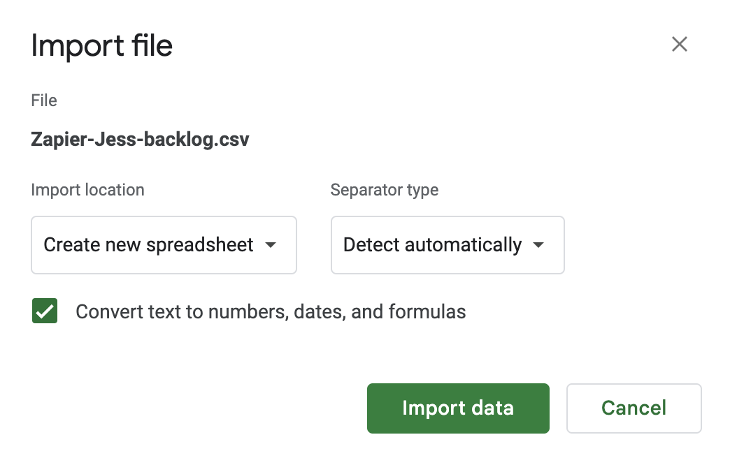
4. Within the Import file popup, you may modify the next: 

   • Import location. This provides you a handful of the way to import your knowledge. For instance, you may import your knowledge into your present sheet, add it as a brand new sheet, or create a brand new spreadsheet altogether. 

   • Separator tab. Google Sheets will robotically detect and apply this, however you can even select a selected sort: Tab, Comma, or Customized. 

     

5. Click on Import knowledge. 

The best way to use the fill deal with in Google Sheets 

The fill deal with in Google Sheets affords a handy option to populate knowledge or copy formulation and knowledge in adjoining cells. Hover your cursor over the bottom-right nook of any cell or cell vary, and it will robotically flip into the fill deal with—it appears to be like like a plus signal (+).

By dragging the fill deal with throughout or down a spread of cells, you may carry out a lot of duties:

1. Copy a cell’s knowledge, together with any formatting, to neighboring cells. 

2. Copy a cell’s method to neighboring cells. 

3. Create an ordered record of information. 

The worth Google Sheets populates within the neighboring cells will range relying on the kind of knowledge contained within the unique cell or cell vary that the fill deal with originated from.  

For instance, if you choose just one cell, the worth of the chosen cell will seem in each cell that you just drag the deal with over. 

If you choose a sequence of neighboring cells, Google Sheets will repeat the sample throughout or down the cells that you just drag the deal with over. Within the instance under, I’ve chosen three neighboring cells, every containing a novel worth: Mango, Coconut, and Pineapple. After I drag the fill deal with, the sample repeats throughout the row in order that it is Mango, Coconut, Pineapple, Mango, Coconut, Pineapple, and so forth. 

If you wish to use the fill deal with to create an ordered record, spotlight at the very least two cells containing the sequence you need Google Sheets to proceed, after which drag the fill deal with. 

On the subject of ordered lists, there’s one caveat value mentioning.  

In contrast to copying textual content values to neighboring cells, Google Sheets will solely proceed sequences for quantity values—not repeat them. For instance, if I needed to repeat the sample Worker 1, Worker 2, Worker 3 throughout the row, Google Sheets would not be capable of. It might simply hold counting up. I must manually copy and paste the values throughout as an alternative. 

To make issues complicated, if I choose a cell vary containing an arbitrary set of numbers—for instance, Worker 1, Worker 17, and Worker 20—Google Sheets would repeat this sample since there isn’t any logical sequence to proceed. 

The best way to robotically import knowledge utilizing Zapier

Do not wish to spend valuable time manually importing knowledge into Google Sheets? Automate the method as an alternative. With Zapier’s Google Sheets integration, you may robotically pull knowledge from different apps into your spreadsheet and orchestrate multi-step, AI-powered workflows. For instance, you may import buyer suggestions from a web based type, use AI to categorize these responses into particular segments or matters, and flag suggestions that meets sure standards for customized follow-up.

Study extra about how one can robotically add knowledge to Google Sheets, or get began with considered one of these pre-made templates.

The best way to use the Google Sheets toolbar

The Google Sheets toolbar is the place you will discover all of your fundamental instruments and formatting choices. Relying on the width of your display screen, among the instruments could also be hidden. To disclose them, click on the Extra icon, which appears to be like like three dots stacked vertically (⋮). 

Hover over any icon to find its perform. Or click on on it to increase that device’s choices, if relevant. Instruments like Borders, Feedback, and Align work equally to what you’d anticipate from Google Docs. 

If you cannot discover a device or wish to examine if a device exists, the quickest option to discover out is by utilizing the search device. Click on the Search the menus icon, which appears to be like like a magnifying glass. 

In contrast to how one can cover the toolbar in Excel, Google Sheets provides you the other capability: you may cover all the pieces above the toolbar, together with the spreadsheet title and tabs, permitting you to concentrate on the spreadsheet itself. To do that, click on the up caret (⋀) within the toolbar or use your keyboard shortcut: Ctrl+Shift+F (on Mac and Home windows). Click on the caret or enter the keyboard shortcut once more to make all the pieces reappear. 

Now again to utilizing the Google Sheets toolbar. 

One of the simplest ways to indicate you how one can use among the most typical Google Sheets formatting instruments is to work via an instance. Let’s edit this easy venture tracker. 

The best way to format knowledge in Google Sheets 

To start out, let’s make the headers within the first row stand out. 

• Click on the cells you wish to format. To use the identical formatting to neighboring cells, choose the primary cell, and drag your cursor throughout or down the cell vary. To use the identical formatting to cells that are not related, choose one cell, press and maintain command on a Mac or Ctrl on Home windows, after which choose the opposite cells. Your cell choice will stay chosen except you click on on a special cell, which is handy if you wish to edit a number of formatting choices. 

• From the toolbar, click on the plus signal (+) subsequent to the font dimension to extend it to 12. Or you may enter 12 within the Font dimension discipline.

• Click on the Daring icon, which appears to be like just like the letter B.  

• Click on the Fill colour icon, which appears to be like like a paint can, and choose a theme colour. I am utilizing a light-weight shade of inexperienced. 

• Click on the Align icon, which appears to be like like a stack of horizontal traces. By default, it is set to Horizontal Align. Click on Middle.

The headings are extra apparent now. However among the heading names are reduce off. Let’s repair that. 

The best way to make Google Sheets cells increase to suit textual content 

There is a default setting in Google Sheets known as Overflow that enables cells with lengthy strings of textual content or numbers to bleed into the neighboring cell. However when you enter knowledge into that neighboring cell, that lengthy string of textual content will get reduce off. 

The simplest option to increase the cell to suit your textual content is by double-clicking the border on the correct aspect of the column you wish to increase. Google Sheets will then increase it to suit the longest worth in that column. 

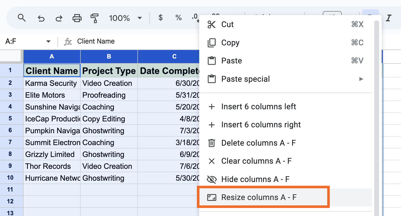
You may as well increase the width of a number of columns directly. 

1. Spotlight the columns you wish to resize. 

2. Proper-click your choice. 

3. Click on Resize columns [names of columns selected]. 

   

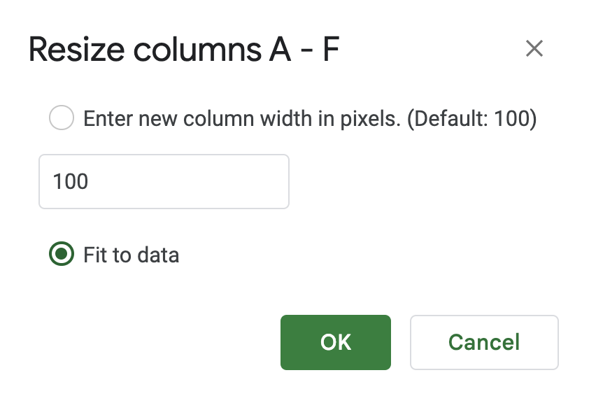
4. Within the Resize columns popup, click on Match to knowledge. 

5. Click on OK. 

   

That is it. No extra smooshed knowledge. 

The best way to wrap textual content in Google Sheets

As an instance you wish to go away your columns a set width. There’s one other method to verify every cell’s knowledge continues to be seen inside a too-small column: wrap the textual content.  

1. Click on the cell or cells you wish to apply the textual content wrap to. 

2. Click on the Textual content wrapping icon within the toolbar, after which choose the Wrap icon. 

3. Google Sheets will robotically change the row peak to suit the info. 

The best way to freeze columns and rows in Google Sheets 

If I scroll down via the venture tracker, the column headers will rapidly disappear from view. To lock the headers in place, let’s freeze the primary row. This is the simplest method to do that. 

1. Within the top-left nook of your spreadsheet, subsequent to column A and above row 1, discover the thick grey bar working horizontally. 

2. Click on and drag the bar underneath the final row you wish to freeze. On this case, that is row 1. 

To unfreeze the row, drag the bar again to its unique place.

You may as well use the identical technique to freeze columns in Google Sheets—simply drag the vertical bar as an alternative. 

The best way to cover columns and rows in Google Sheets

If you’re working with infinite rows of information, it is simple to lose observe of what is what. A technique that can assist you focus is by quickly hiding any rows of irrelevant knowledge.  

1. Spotlight the rows or columns you wish to cover. 

2. Proper-click your choice. 

3. Click on Cover rows [numbers of rows selected]. 

You may know rows are hidden if there are numbers lacking out of your row headers. Or, within the case of columns, lacking column letters.

To make the rows seen once more, click on the arrows that seem in lieu of the hidden rows. 

The best way to add a sheet in Google Sheets

You may add one other sheet to your current spreadsheet utilizing considered one of two strategies: add a brand new clean sheet or duplicate and current one. This is how one can do each.

The best way to add a brand new clean sheet

If you wish to add a clean sheet to your current spreadsheet, click on the Add sheet icon, which appears to be like like a plus signal (+), on the backside of your current spreadsheet. 

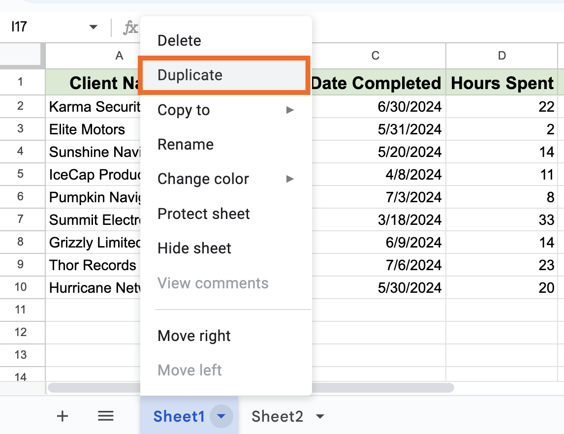
The best way to duplicate a Google Sheet

You may as well make a duplicate of a sheet in Google Sheets. 

1. Click on the down caret (⋁) subsequent to the tab with the title of the sheet you wish to duplicate. 

2. Click on Duplicate. 

   

3. Double-click the sheet’s tab to rename it. 

The best way to use Google Sheets formulation

Like most spreadsheet apps, Google Sheets affords a bunch of built-in formulation that can assist you course of a lot of statistical and knowledge manipulation duties. You may as well mix formulation to create extra highly effective calculations and string duties collectively. In case you’re already accustomed to crunching numbers in Excel, many of the formulation work in Google Sheets the very same method. 

As a refresher, a perform is a predesigned method that is constructed into the app, whereas a Google Sheets method is any equation you give you. Earlier than you spend time creating new formulation, it is useful to know which capabilities are already out there. 

This is a fast overview of the commonest fundamental Google Sheets capabilities. 

• SUM: provides all of the values in a cell vary. For instance, =SUM(D2:D10) in our spreadsheet would add up all of the hours spent throughout cells D2 to D10. 

• AVERAGE: returns the common of a spread of cells. For instance, =AVERAGE(D2:D10) would return 16. 

• COUNT: counts the variety of cells in a given vary that comprise numbers. For instance, =COUNT(D2:D10) would return 9 as a result of each cell in that vary incorporates a quantity. If I deleted the worth in cell D5, the rely would robotically change to eight.

• MAX: returns the very best worth in a cell vary. For instance =MAX(D2:D10) would return 33. 

• MIN: returns the bottom worth in a cell vary. For instance, =MAX(D2:D10) would return 2.

You may as well flick thru Google Sheets’s intensive library of capabilities for an entire breakdown.  

The best way to use Google Sheets capabilities 

There are two most important methods to make use of a Google Sheets perform.

Enter the perform title within the cell 

One option to insert a perform in a cell is to enter the equal signal (=) instantly adopted by the perform title. Google Sheets will autocomplete the perform title and recommend what knowledge you must embody within the perform. For instance, once I enter =SUM in cell E12, Google Sheets finishes the method by suggesting =SUM(E2:10). Google Sheets will even recommend an inventory of different associated capabilities. To simply accept the prompt method, press Tab. 

Another choice: After you enter =, click on Generate method with Gemini within the dropdown. From there, you may ask Gemini to create a method for you utilizing plain English—for instance, “Inform me which venture generates essentially the most quantity billed, on common.”

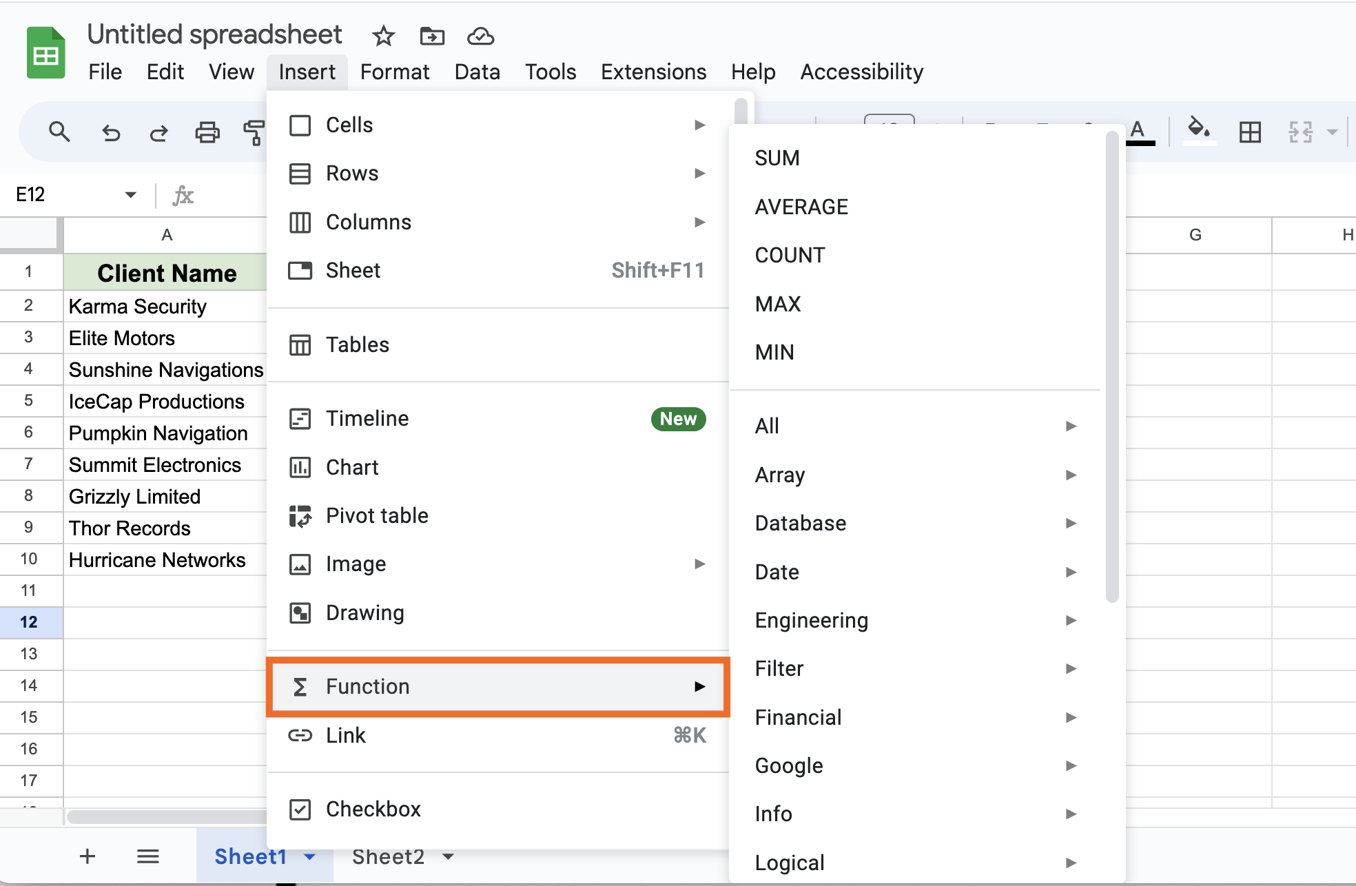
Select from the Perform menu 

1. Click on the cell you wish to enter the perform into. 

2. Click on Insert, after which choose Perform. 

3. Click on the perform you wish to use. 

   

4. Google Sheets will populate the perform in your cell, together with the parentheses the place you will have to enter your argument—the knowledge you need the method to calculate. For instance, within the method =SUM(E2:E10), the argument E2:E10 tells Google Sheets so as to add the values of cells E2 to E10. 

Now let’s get again to how one can use Google Sheets formulation. 

To create a method to calculate easy arithmetics, like including, subtracting, or multiplying, you must use particular symbols. 

• So as to add: use the + signal.

• To subtract: use the - signal.

• To multiply: use the * signal.

• To divide: use the / signal.

• To make use of exponents: use the ^ signal.

Keep in mind: Each method should start with an equal signal (=) instantly adopted by the method. By default, Google Sheets will use PEMDAS to find out the order of operations (what to calculate and in what order): Parentheses first, adopted by Exponents, Multiplication, Division, Addition, after which, lastly, Subtraction. 

For instance, if I enter =10-5*2, Google Sheets will return 0. But when I enter =(10-5)*2, it’s going to return 10.

If in case you have a sequence of calculations that have to occur in a selected order, use PEMDAS. 

The best way to create a pivot desk or chart in Google Sheets 

Now that you understand how to create a spreadsheet, import knowledge, and use formulation, let’s go over extra superior methods to control and visualize your knowledge. 

The best way to create a pivot desk in Google Sheets

A pivot desk is a useful option to analyze giant knowledge units. With a pivot desk, you need to use the identical knowledge, manipulate it nevertheless you need, and get new insights every time—you do not have to create a brand new spreadsheet for every evaluation. 

We’ve an in-depth tutorial on how one can create and use pivot tables in Google Sheets, however this is a fast overview. 

1. Choose all the cells with the supply knowledge that you just wish to use, together with column headers. 

2. Click on Insert, and choose Pivot desk. 

3. Select if you wish to insert your desk into a brand new sheet or an current one. 

4. Within the pivot desk editor, add the rows and columns you wish to analyze, together with the values you wish to show inside every row and column.  

The information in your pivot desk will robotically change if the supply knowledge modifications. In case you do not see the modifications mirrored in your pivot desk, refresh your web page. It could take a minute to replace, relying on the quantity of information modifications.

The best way to create a chart in Google Sheets 

As an instance I wish to rapidly visualize how a lot time every consumer spent on their venture. A technique to do that could be to create a chart. 

1. Choose all the cells with the supply knowledge you wish to use, together with column headers.

2. Click on Insert, after which choose Chart. 

3. By default, Google Sheets will flip your knowledge right into a bar graph, and, for some odd purpose, it’s going to place that graph immediately on prime of your supply knowledge. To switch the chart or to make use of a special sort altogether, use the Chart editor. Alternatively, you may inform Gemini (the immediate bar’s on the prime of the aspect panel) what sort of chart you wish to create, and it will maintain the remainder.

4. Click on any of the blue dots surrounding the border of your chart to resize it. You may as well drag and drop the chart to reposition it. 

If you wish to make extra edits afterward, right-click the chart and choose the sphere you wish to edit. Clicking any discipline will carry the complete Chart editor again into view. 

The best way to share and collaborate in Google Sheets 

There are just a few methods to share your spreadsheet, however this is the simplest one: 

1. Click on Share above your spreadsheet. 

2. Within the Share popup, you may: 

3. Any particular person you give spreadsheet entry to will robotically have full Editor permissions—they’ll make modifications, go away feedback, and provides others entry to the file. To vary this, click on Editor subsequent to their title and select their permission degree: Viewer or Commenter. You may as well set an entry expiration date from right here.

4. Click on Save. 

Along with sharing with particular individuals, you can even give common entry to anybody in your group or anybody with the hyperlink. 

Phrase of recommendation: In case your spreadsheet incorporates cell ranges that should not be tampered with, lock cells in Google Sheets earlier than sharing it. 

Automate Google Sheets with Zapier

Google Sheets is commonly the spine of how groups retailer and manage knowledge, however the actual worth comes while you use that knowledge to energy the remainder of what you are promoting’s workflows. Wen you utilize Zapier’s Google Sheets integration, you may orchestrate multi-step, AI-powered workflows that flip a static spreadsheet into half of a bigger system.

For instance, each new on-line order in your eCommerce website might be robotically logged in Google Sheets, then handed via ChatGPT to generate a customized thank-you observe, enriched with CRM knowledge to incorporate loyalty standing, after which routed via your e-mail platform for supply.

Uncover extra methods to automate Google Sheets, or get began with considered one of these pre-made templates.

Associated studying: 

This text was initially printed in July 2016 with contributions from Michael Grubbs and Shea Stevens. The newest replace was in September 2025.