Tips on how to use VLOOKUP in Excel

While you’re observing limitless rows of knowledge in an Excel spreadsheet, it is simple for all that info to show into one blurry mess. Then there’s the matter of extracting particular information. Along with spending what seems like an eternity scrolling by the spreadsheet to search out what you want, you then second-guess when you really pinpointed the proper information. 

That is the place VLOOKUP in Excel is available in: it takes the guesswork out of discovering and retrieving information in spreadsheets. 

This is the brief model of use VLOOKUP in Excel (maintain scrolling for extra particulars).

1. Click on the cell the place you need Excel to return the info you are searching for. 

2. Enter =VLOOKUP(lookup worth,desk array,column index quantity,vary lookup).

3. Press Enter or return.  

Desk of contents:

What’s VLOOKUP in Excel? 

VLOOKUP in Excel is a built-in perform that searches for a worth in a single column primarily based on a given worth in one other column. The components is made of 4 parameters (or arguments): 

• Lookup worth: That is the worth you need Excel to seek for. Notice: The lookup worth should be within the first column within the given vary. For instance, in case your lookup worth is in cell A3, then your vary ought to begin with A. 

• Desk array: That is the cell vary containing the lookup worth and the worth you need Excel to return (the info you are searching for).

• Column index quantity: That is the column quantity within the given vary containing the worth you need Excel to return. In case your desk array is A2:D10, for instance, depend column A as your first column, column B as your second, and so forth. In case your desk array is C2:F10, depend column C as your first column, column D as your second, and so forth. Your column index quantity tells Excel which column to retrieve the info you are searching for. 

• Vary lookup: That is an optionally available parameter. By default, the VLOOKUP perform all the time returns an approximate match (designated by TRUE). If you’d like a precise match, enter FALSE.  

Put these parameters collectively and also you get this VLOOKUP components:  

=VLOOKUP(lookup worth,desk array,column index quantity,vary lookup)

Tips on how to use VLOOKUP in Excel 

This is an in depth breakdown of use VLOOKUP (or vertical lookup). Notice: I am utilizing Excel on-line, however the steps are the identical within the desktop app.

To maintain this tutorial easy, I am going to present you use the VLOOKUP perform in Excel to establish an worker’s ID primarily based on their final identify—on this case, it is Kwon. When you’d most likely use VLOOKUP for one thing extra complicated with a a lot bigger dataset, the steps to make use of VLOOKUP stay the identical. 

A fast reminder: the lookup worth should be within the first column of your desk array. For this demo, our lookup worth (Kwon in cell B6) shall be within the first column of our desk array (B2:D10). In case you’re working with a special dataset the place the lookup worth is not within the first column, you could have to reorganize your information. Or you’ll be able to copy and paste the columns you are working with into one other space of your worksheet. In case you go together with the latter, I like to recommend pasting the info into a brand new worksheet altogether to maintain your information manageable.

As soon as your information is organized, you are able to get began. 

1. Click on the cell the place you need Excel to return the info you are searching for. On this case, click on cell B13.

2. Enter =VLOOKUP. 

3. Press Enter or return. Excel will robotically add a left parenthesis after the perform, so it seems to be like this: =VLOOKUP(. 

4. Enter the next parameters instantly after the parenthesis, separating every one with a comma. 

   • Lookup worth: B6

   • Desk array: B2:D10

   • Column index quantity: 3 (Bear in mind: the worth we wish Excel to return [employee ID] is in column D, which is the third column of the given cell vary.)

   • Vary lookup: Enter FALSE to get a precise match

5. Enter the proper parenthesis ) to shut your components in order that cell B13 now reads =VLOOKUP(B6,B2:D10,3,FALSE).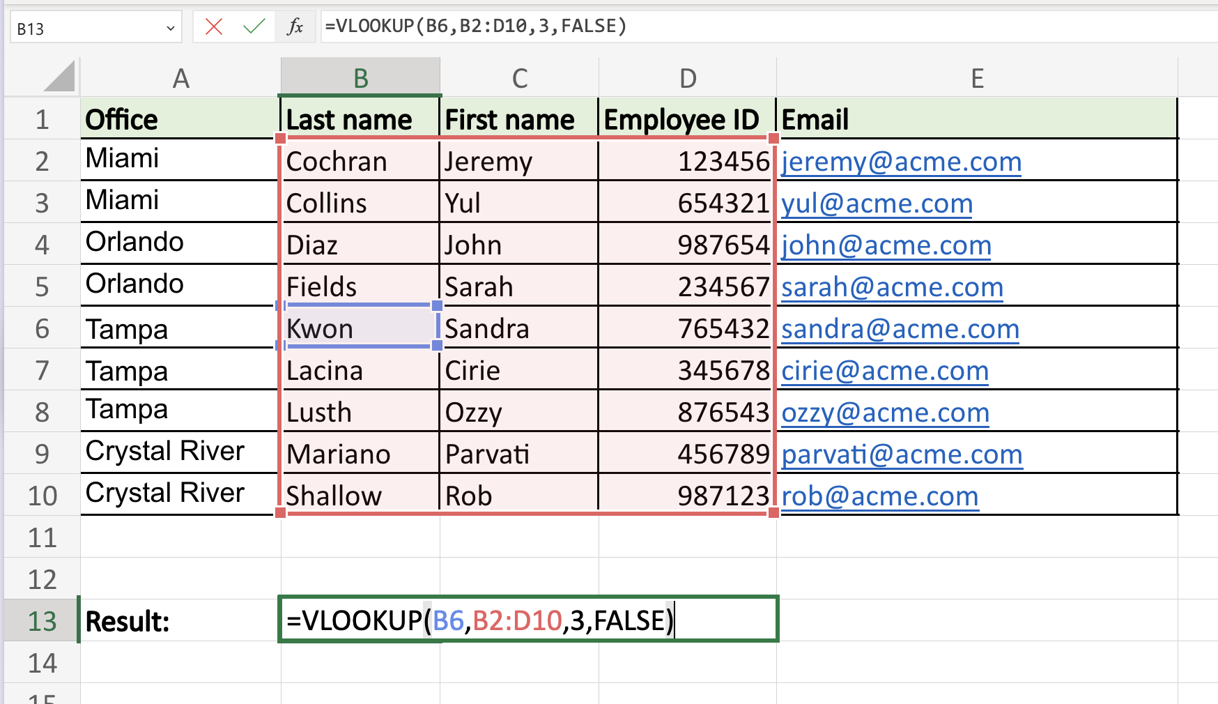 

   

6. Press Enter or return. 

   

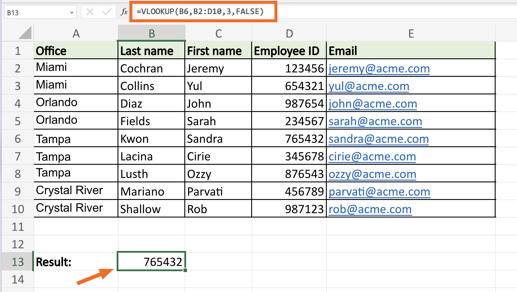
Excel instantly returns the corresponding worth: 765432.

Tips on how to do VLOOKUP in Excel with two spreadsheets

As an instance Sheet 1 of our demo workbook is our main spreadsheet—it accommodates each little bit of worker information. There’s additionally a second spreadsheet (Sheet 2), which accommodates solely worker names and their up to date firm electronic mail addresses. 

Now you should replace the e-mail addresses in Sheet 1 with the brand new electronic mail addresses from Sheet 2. You may accomplish this with the VLOOKUP perform, however you will want to change your desk array parameter to inform Excel which spreadsheet accommodates the corresponding lookup worth you need it to return. 

That is the modified VLOOKUP components to return a worth from one other sheet throughout the similar workbook: 

=VLOOKUP(lookup worth,sheet!vary,column index quantity,vary lookup) 

Let’s use VLOOKUP to replace the e-mail deal with in cell E2 of Sheet 1 with the e-mail deal with in cell C2 of Sheet 2. 

1. Click on cell E2 of Sheet 1.

2. Enter =VLOOKUP(B2,Sheet2!$A$2:$C$10,3,FALSE). This is a breakdown of the modified desk array: 

   • Sheet2!: That is the identify of the spreadsheet that accommodates the given cell vary. Notice: to reference one other worksheet, enter [name of sheet]!. In case your sheet identify accommodates areas or non-alphabetical characters, it should be enclosed in single citation marks. For instance, 'Sheet 1'!.

   • $A$2:$C:$10: The cell vary is A2:C10. To forestall the vary from altering when copying the components to different cells, we lock it in utilizing absolute cell references. 

3. Press Enter or return. 

Excel returns the corresponding worth from Sheet 2 in cell E2 of Sheet 1: j.cochran@acme.com. 

To rapidly replace the remaining electronic mail addresses in Sheet 1, drag the fill deal with from cell E2 down. 

Tips on how to do VLOOKUP in Excel with two workbooks

To make use of VLOOKUP to retrieve information from one other workbook, all it’s a must to do is embody the file identify of the opposite workbook inside sq. brackets instantly adopted by the sheet identify and desk array. This is the components template: 

=VLOOKUP(lookup worth,[file_name.xlsx]Sheet!vary,column index quantity,vary lookup)

As an instance we saved the workers’ up to date electronic mail addresses in Sheet 1 of the 2023_employee_emails.xlsx workbook as an alternative. To populate the brand new electronic mail deal with in cell E2 of our main spreadsheet, enter: 

=VLOOKUP(B2,[2023_employee_emails.xlsx]Sheet1!$A$2:$C$10,3,FALSE)

Tips on how to use VLOOKUP in Excel with Copilot

In case you’ve made it this far with out rage-quitting Excel and going to reside off the grid in Saskatchewan, I’ve a reward for you: you should utilize Copilot, Microsoft’s built-in AI assistant, to construct the VLOOKUP components for you. 

Earlier than you get too excited, maintain the next in thoughts: 

• You need to use this function solely if in case you have a Copilot Professional subscription or a Microsoft 365 Private or Household subscription that features Copilot. 

• Copilot works solely with Excel information saved on OneDrive or SharePoint with AutoSave turned on. 

• Remember to format your information as tables (Copilot does not work with common ranges). 

Now, let’s dive in. 

1. Along with your workbook open, click on Copilot on the ribbon to open a brand new chat. Or click on any cell and choose the Copilot icon that seems subsequent to it. 

2. Describe what you want within the message bar. For instance, “Write a VLOOKUP components to drag electronic mail addresses from Desk A to Desk B.” The extra particular your AI immediate, the higher. 

3. Copilot will generate a components, together with a preview of the outcomes, and show it within the chat. 

4. Optionally, immediate Copilot to tweak the components till it is precisely what you want. 

5. Hover over Insert column beneath the outcomes preview to view the outcomes immediately in your sheet. If it seems to be good, click on Insert column. Alternatively, you’ll be able to copy and paste the components your self.

It is that straightforward. Simply do not inform your previous self, who’s nonetheless weeping right into a spreadsheet in 2013.

Automate Excel with Zapier

Handbook information entry does not scale—and it is simple to get improper. With Zapier as an orchestration layer, you’ll be able to join Excel with hundreds of different apps and orchestrate how information flows throughout your tech stack. For instance, robotically log new occasion suggestions in Excel, use AI to categorize the suggestions sort and analyze buyer sentiment, and ship a abstract of the evaluation to your staff in Slack or through electronic mail.

Study extra about automate Excel, or strive one in all these pre-made templates to get began.

Associated studying: 

This text was initially revealed in July 2019 by Khamosh Pathak. The newest replace was in August 2025.